Disentangling the Good From the Bad: Quantization-Induced Flips Are Not Random

Bouguerra, Aymen; Arnez, Fabio; Gomez-Villa, Alexandra; Mraidha, Chokri

NeurIPS 2026 (A*) · Main Conference Paper

Advances in Neural Information Processing Systems

Disentangling the Good From the Bad:
Quantization‑Induced Flips Are Not Random

Aymen Bouguerra¹
Fabio Arnez¹
Alexandra Gomez-Villa^2,3
Chokri Mraidha¹

¹Université Paris-Saclay, CEA-List · ²Computer Vision Center, Spain · ³Universitat Autònoma de Barcelona

Paper coming soon Code CEA-List BibTeX

Three panels on pooled CLIP-B/16 W8A8 QAT flips. (A) Densities of the quantized top-1 margin for good and bad flips overlap. (B) Share of flips by the SVD rank at which the quantized prediction emerges: good flips peak at low ranks (median 24), bad flips rise in the high-rank tail (median 48). (C) A confidence score against a spectral score: the two populations form largely separate clouds. — **Quantization flips are not random** (pooled CLIP-B/16, W8A8 QAT, 8 datasets, 13,205 flips). **(A)** The quantized softmax margin used by prior work overlaps for good (IC) and bad (CI) flips. **(B)** Along the SVD rank of the quantized model's own feature space, good flips emerge at low ranks and bad flips need the high-rank tail. **(C)** A confidence score and a spectral score together largely disentangle the two populations.

TL;DR

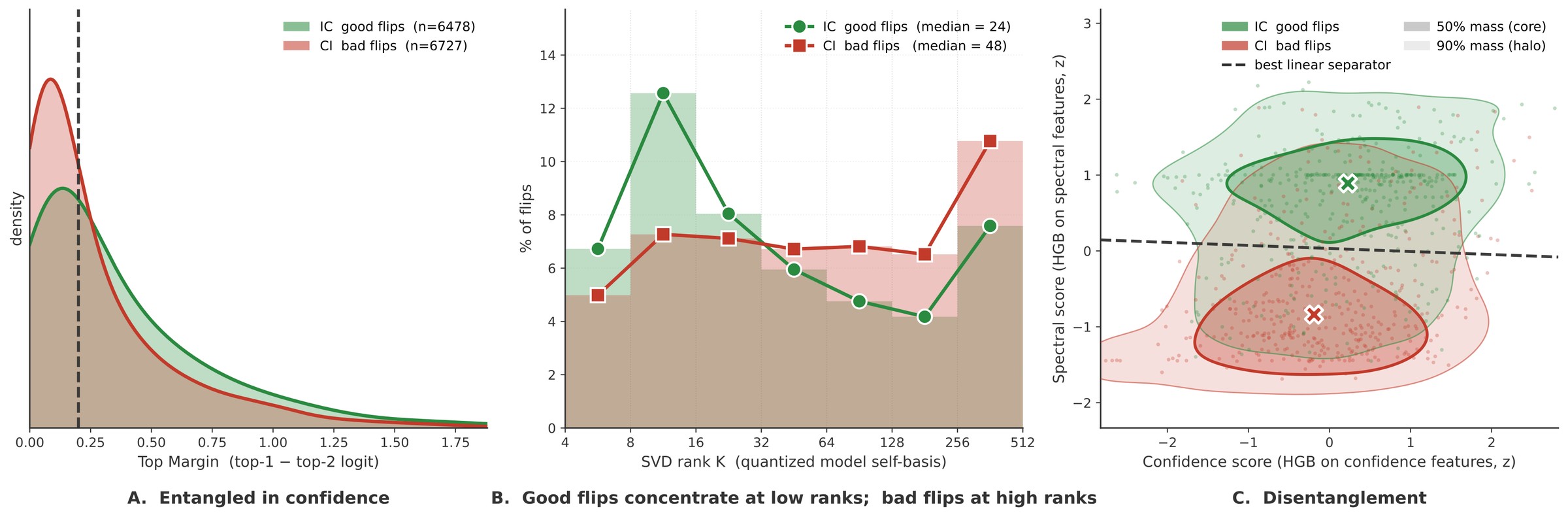
A quantized model that matches its full-precision baseline in accuracy still changes many of its predictions. These flips are not rounding noise: good flips (incorrect → correct) and bad flips (correct → incorrect) live in different parts of the quantized model's SVD spectrum. A post-hoc gate that reads them can keep the good flips and repair the bad ones, recovering accuracy at a cost of microseconds per input.

0.881

Dis AUC on 50 CLIP cells

T3; 0.775 from the quantized model alone (T1)

+1.97 pp

Accuracy gain, quantized model alone

T1 on the 50 CLIP cells; +0.86 pp above full precision

+3.42 pp

Above full precision after a −2.88 pp drop

T3, TensorRT INT8, CLIP-L/14 / GTSRB

0.045%

Gate compute vs a quantized forward

T1, mean over the 50 CLIP cells; no second model in memory

Abstract

Model quantization has advanced tremendously in recent years, producing models that require a fraction of the compute while maintaining baseline accuracy and creating the illusion of lossless compression. Beneath the surface, however, model behavior undergoes severe shifts that simple global accuracy fails to capture. Notably, quantized models experience a high rate of “flips”: individual predictions that change from correct to incorrect (bad flips-CI) and vice versa (good flips-IC). Although overall accuracy remains stable, these changes degrade model reliability and introduce unforeseen safety risks. Current literature attributes these flips to random rounding noise, a perspective that ignores the specific precision constraints imposed by quantization with or without training.

In this paper, we show that flips are driven by quantization's implicit regularization, low-pass filtering, and exacerbated spectral bias. By analyzing these effects via Singular Value Decomposition (SVD), we leverage the model's low-to-high rank internal disagreement to disentangle good flips from bad ones. Building on this insight, we introduce learned post-hoc gates, with or without the full-precision model, to selectively preserve the former while correcting the latter, and we validate our disentanglement through experiments spanning Post-Training Quantization (PTQ) to Quantization-Aware Training (QAT) and across vision, language, and multi-modal models. With this work, we aim not only to restore the quantized model's hidden reliability degradation but also to elevate it beyond the accuracy ceiling of its full-precision counterpart.

The problem

Matched accuracy still changes many predictions

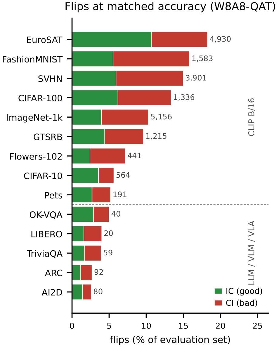
When a quantized model matches its baseline's top-1 accuracy, the two are treated as equivalent. They are not: at matched accuracy, the quantized model still disagrees with its baseline on a share of inputs. Good and bad flips are roughly symmetric in count, which is exactly why the aggregate accuracy gap looks small or even null.

The quantized model's own confidence does not tell them apart: their densities overlap across the whole confidence range. Without a per-input criterion, a deployed model cannot flag the bad flips that matter, such as a missed pedestrian or a corrupted instruction.

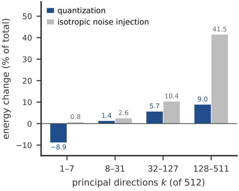
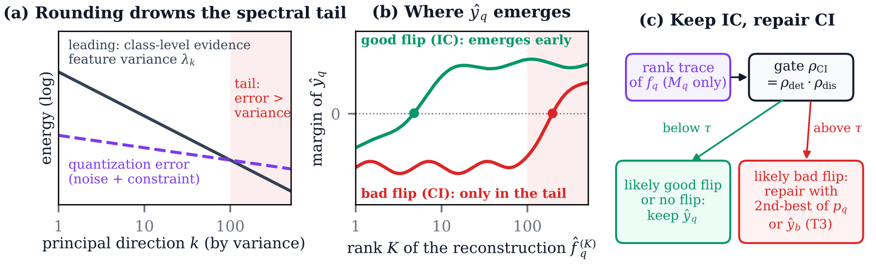
The spectral account explains the asymmetry. Rounding error concentrates in the high-rank, low-variance directions of the representation, which carry fine within-class cues. A good flip is an input where the baseline followed a misleading high-rank cue that quantization removed; a bad flip is one whose correct evidence lived in that tail and was crushed by rounding.

Bar chart of good and bad flip counts per dataset at matched accuracy, for vision, text and text-vision models; bar length is the flip share of the evaluation set, from about 3 to 18 percent, and each bar is labelled with its flip count. — Good (IC) and bad (CI) flips at matched accuracy across vision, text and text-vision models. Bar length: flip share of the evaluation set; labels: flip counts.

Bar chart of the signed energy change per rank range of the full-precision basis under quantization, against isotropic noise of equal drift energy: quantization removes energy from the leading ranks and adds far less to the high-rank tail than noise does. — **Quantization is not isotropic noise.** Signed energy change per rank range of *V_b* (share of total; CLIP-B/16 W8A8 PTQ, CIFAR-10) vs isotropic noise of equal drift energy. Ranks 1–7 lose 8.9%; ranks 128–511 gain 9.0% (noise: 41.5%), yet drift there is 1.5× their own energy.

Method

Read where each prediction emerges, then gate

The active basis V_q is the SVD of the quantized model's own features, fitted without labels and without the full-precision model. For each input, rank-K reconstructions of its feature are pushed through the classifier head on a grid of ranks: the readouts trace, rank by rank, where the quantized prediction emerges. Together with the softmax statistics they form the feature set of two gradient-boosted heads (a flip, and a bad one), fitted once with labels on a calibration pool. The deployed gate multiplies their scores, flags the inputs most likely to be bad flips and repairs only those.

Three-panel schematic. (a) Along the principal directions, rounding error overtakes the variance in the low-variance tail while the leading directions keep the class-level evidence. (b) Probability of the quantized prediction against the rank K of the reconstruction: a good flip emerges early and stays, a bad flip emerges only in the high-rank tail. (c) The gate keeps inputs scored as good flips or non-flips and repairs likely bad flips. — **Why good and bad flips separate by rank** (schematic). **(a)** Rounding adds a noise component and a precision-grid constraint; along the principal directions, its error overtakes the variance in the low-variance tail, where fine within-class cues live, while the leading directions keep the class-level evidence. **(b)** A good flip is carried by the leading directions, so *ŷ_q* becomes and stays the argmax of the rank-K reconstruction at a low K; a bad flip is decided in the drowned tail and emerges only at high K. **(c)** The gate reads this rank trace from *M_q* alone, keeps inputs scored as good flips or non-flips, and repairs likely bad flips with the second-best class of *p_q* (T1/T2) or *ŷ_b* (T3).

Method overview. (A) The full-precision and the quantized model produce features and predictions; joint correctness defines the outcomes C, CI, IC and I/II; the active basis is the SVD of the quantized features, read on a rank-K grid. (B) Three deployment tiers: T1 uses the quantized model only and repairs flagged inputs with the second-best class; T2 adds a cached full-precision basis to the features; T3 runs the full-precision model on the flagged inputs. — **Method overview.** **(A)** Notation: *M_b* (full precision) and *M_q* (quantized) produce features and predictions; joint correctness defines the outcome, and IC and CI are the flips. **(B)** Three tiers that differ only in what they may query of *M_b* at inference: T1 and T2 never run it, T3 does.

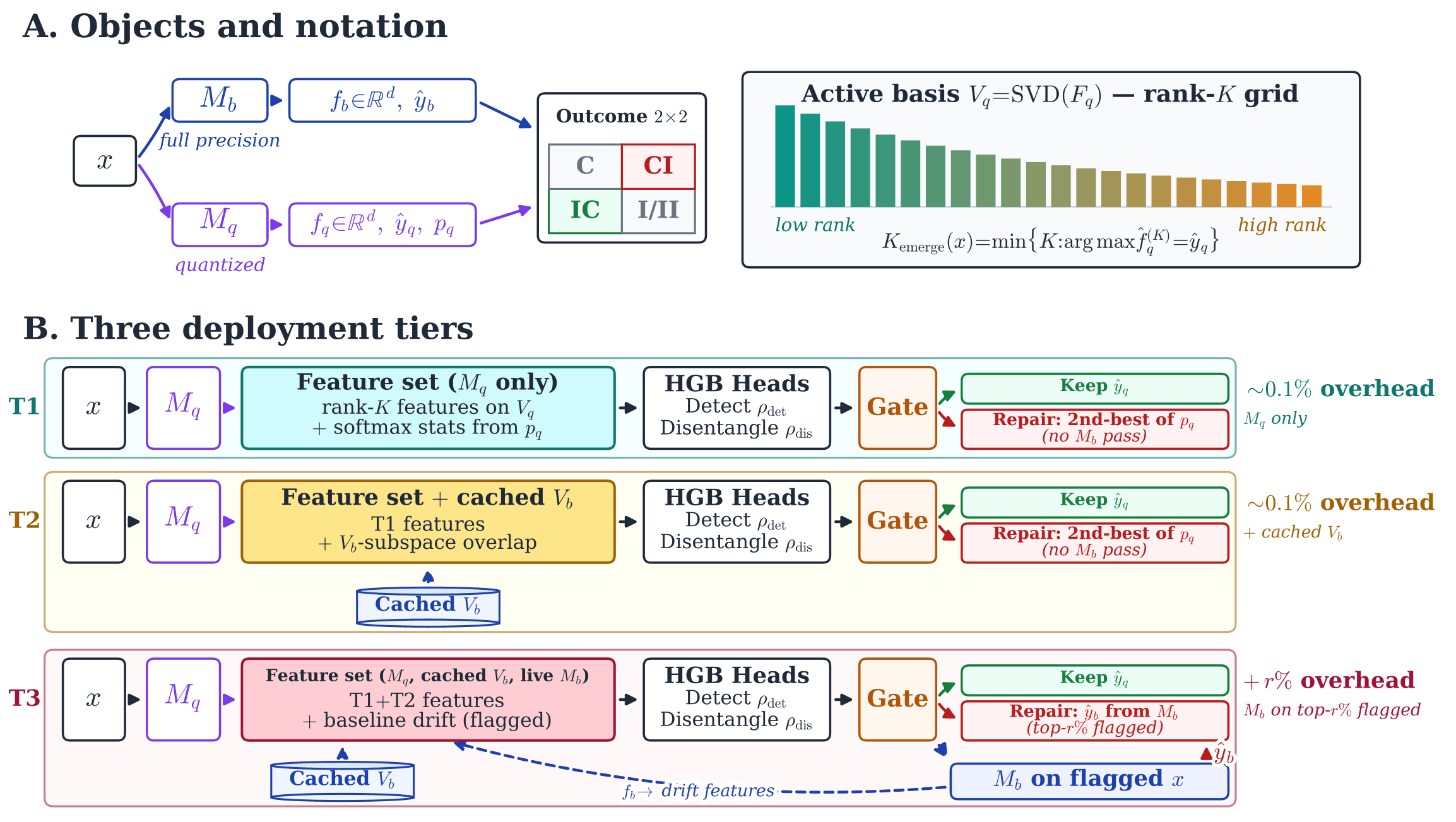
Configuration	Gate features	Repair of flagged inputs	M_b forwards / input
T1	M_q only (V_q readouts, p_q)	second-best class of p_q	0
T2	T1 + cached V_b	second-best class of p_q	0
T3	T1/T2 gate, then live M_b on its top-r%	ŷ_b (T3 head) or T1/T2's	r

r: flag rate. The second-best class of p_q equals the label for about three quarters of bad flips and essentially no good flips, so a flagged input can be repaired without a full-precision pass. The T1 / T2 gate adds 0.045–0.053% of a quantized forward in compute (mean over the 50 CLIP cells); T1 uses the quantized model only.

Algorithm 1 The deployed gate. B_T1/T2/T3: the tiers' feature sets; T1 and T2 never run M_b. In the reported gains, P is the evaluated set, scored out-of-fold (5 folds), and T2 keeps the better of the T1 and T2 gates.

Calibration (once, on a labelled set P)

Run M_q and M_b on P; V_q ← SVD of the centred F_q; cache (μ_b, V_b) from F_b
For each tier set B_T1, B_T2, B_T3: fit ρ_det (HGB on 1[ŷ_q ≠ ŷ_b], all of P), ρ_dis (HGB on 1[CI], flipped inputs of P), and ρ_CI ← ρ_det · ρ_dis; T3's is ρ_CI^T3
Pick the repair rate r_q, then k, by accuracy gain on P; τ, τ_b ← (1 − r_q)- and (1 − r)-quantiles of ρ_CI (r: M_b rate of T3); τ₃ ← (1 − k)-quantile of ρ_CI^T3 over the inputs with ρ_CI ≥ τ_b

Inference (per input x)

ŷ_q, p_q, f_q ← M_q(x); z ← B_T1(f_q, p_q, V_q) or B_T2(f_q, p_q, V_q, μ_b, V_b)
ỹ ← ŷ_q not flagged: output untouched
if ρ_CI(z) ≥ τ: ỹ ← second-best class of p_q T1, T2: M_q only
T3: if ρ_CI(z) ≥ τ_b: run M_b(x) M_b on r of the inputs
if ρ_CI^T3(B_T3(x)) ≥ τ₃: ỹ ← ŷ_b else ỹ is kept
return ỹ

Disentanglement

The signal holds across 50 CLIP cells and four more families

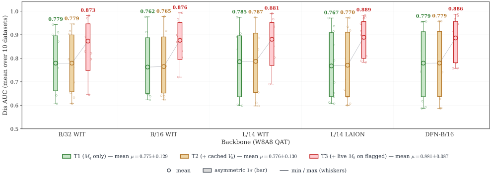
Dis AUC is the ROC-AUC separating good from bad flips among the flipped inputs. On five CLIP backbones × ten datasets at matched-accuracy W8A8, T3 sits between 0.87 and 0.89 for every backbone. T3 is the best tier on every family tested, and T2 adds nearly nothing beyond T1: the cached full-precision directions are the same for every input, so fresh per-sample evidence arrives only through a full-precision forward pass.

Box plot of disentanglement AUC per CLIP backbone and tier over ten datasets: T1 means from 0.762 to 0.785, T2 about equal, T3 from 0.873 to 0.889. — **Disentanglement AUC per CLIP backbone** (W8A8 QAT, ten datasets each; extended feature set). Pooled means: T1 0.775, T2 0.776, T3 0.881.

Family	#	T1	T2	T3
VLMs (5 × CLIP)	50	0.775	0.776	0.881
Generative VLMs	2	0.749	0.745	0.751
ViT-B/16	3	0.802	0.802	0.828
CNN ResNet-50	3	0.683	0.692	0.707
LLMs	3	0.676	0.687	0.702

Family-averaged Dis AUC; # = number of (model, dataset) cells.

Detection comes first

Deployment also needs to find the flips against a low base rate (8.7% of 47,636 inputs). The M_q-only gate reaches PR-AUC 0.535, 6.1× the prior, at under 0.1% overhead; spending a full-precision pass on the top 10% flagged inputs lifts it to 0.851, and the top 20% to 0.958.

Tier	Overhead vs M_q	PR-AUC	ROC-AUC	Recall at P = 50%	Recall at P = 60%
T1 (M_q only)	< 0.1%	0.535	0.936	63.3%	34.3%
T2 (+ cached V_b)	< 0.1%	0.567	0.940	67.3%	42.0%
T3 (M_b on the top-r% flagged), varying the flag rate
r = 1%	+1.0%	0.609	0.942	69.2%	46.8%
r = 5%	+5.0%	0.744	0.956	79.7%	66.8%
r = 10%	+10.0%	0.851	0.972	88.8%	81.7%
r = 20%	+20.0%	0.958	0.991	96.6%	94.9%
r = 50%	+50.0%	0.998	0.999	99.7%	99.7%

Flip detection on the CLIP B/16 + B/32 CC3M-QAT set (N = 47,636, flip prior 0.087, 5-fold CV, mean of five QAT runs).

Class density caps T1, softly

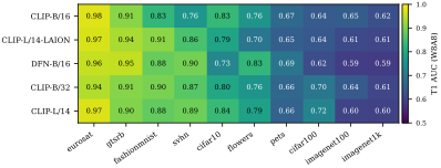
Low-class datasets (EuroSAT, GTSRB, FashionMNIST, SVHN) form a bright band at 0.76–0.98, while ImageNet-1k caps T1 at 0.59–0.62: with 1,000 classes in a fixed feature space, quantized-model-only features can no longer tell which low-rank reconstruction matches which class. A live M_b pass on flagged inputs (T3) lifts ImageNet-1k from 0.60 to 0.79, and tighter precision lifts it too, to 0.829 / 0.847 at W4A4 (ResNet-50 / ViT-B/16).

Heatmap of T1 Dis AUC for five CLIP backbones by ten datasets at W8A8: values from 0.83 to 0.98 on EuroSAT, GTSRB and FashionMNIST, falling to 0.59 to 0.62 on ImageNet-1k. — **T1 Dis AUC**, five CLIP backbones × ten datasets, W8A8; rows and columns sorted by mean.

Backbone	T1 W8A8	T3 W8A8	T1 W6A8	T3 W6A8
CLIP-B/32 WIT	0.779	0.873	0.761	0.879
CLIP-B/16 WIT	0.762	0.876	0.770	0.883
CLIP-L/14 WIT	0.785	0.881	0.769	0.879
CLIP-L/14 LAION-2B	0.767	0.889	0.772	0.884
DFN-B/16	0.779	0.886	0.766	0.882

Mean Dis AUC over the ten datasets of each backbone (extended feature set).

Repair

Keep the good flips, repair the bad ones

Two heads flag the inputs most likely to be bad flips (a flip, and a bad one); each tier repairs them from its cheapest source. On the 50 CLIP cells (5 backbones × 10 datasets, W8A8 light QAT), T1 gains +1.97 pp with the quantized model alone and ends +0.86 pp above full precision. T3 runs the full-precision model only on the flagged inputs and climbs with that budget.

	T1	T2	T3 r=1%	T3 r=5%	T3 r=10%	T3 r=17%	T3 r=20%	T3 r=50%	T3 r=70%	Oracle
Repair	2nd-best	2nd-best	ŷ_b where the T3 head picks, else T2's repair							ŷ_b
Top-1 accuracy gain (pp)
above the quantized model	+1.97	+2.03	+2.11	+2.44	+2.77	+3.10	+3.19	+3.70	+3.74	+4.83
above the base model (FP)	+0.86	+0.92	+1.01	+1.33	+1.66	+1.99	+2.08	+2.59	+2.64	+3.72
Compute overhead (% of M_q)	0.045	0.053	1	5	10	17	20	50	70	4.8

Mean over the 50 cells. T1 / T2 never run the full-precision model; T3 runs it only on the r% of inputs the T1/T2 gate flags. Each gain takes the best flag rate on the evaluated cells, an upper estimate for a deployment that fixes r in advance. Compute overhead: FLOPs as a percentage of one quantized forward; for T1 / T2, the feature set and both heads (at most 0.57%, on B/32 ImageNet-1k).

Deployment

Every production quantizer gains

The pipeline on production quantizers: GPTQ, SmoothQuant, AWQ and the stock recipes of NVIDIA TensorRT Model Optimizer for zero-shot CLIP on GTSRB, plus quantized LLMs and VLMs (QAT, bitsandbytes-INT8, TensorRT). With a 2–5 pp drop, T1 recovers 2.9–3.6 pp and T3, which runs the full-precision model on 20% of the inputs, 5.2–6.3 pp, ending up to 3.4 pp above full precision.

Model	Data / Quant	Quant. loss Δ (pp)	Flips after (before)		PR-AUC (random)	Dis AUC		Gain (pp)
Model	Data / Quant	Quant. loss Δ (pp)	Good	Bad	PR-AUC (random)	T1	T3	T1	T3
(a) Little or no damage on CLIP / GTSRB (\|Δ\| < 1 pp)
CLIP-B/32	GPTQ W8A8	+0.07	406 (459)	210 (450)	0.638 (0.228)	0.768	0.896	+2.28	+2.79
CLIP-B/32	TRT INT4-AWQ	−0.32	321 (337)	191 (350)	0.872 (0.530)	0.750	0.917	+1.57	+3.93
CLIP-B/32	TRT INT8-SQ	−0.02	149 (171)	94 (172)	0.718 (0.276)	0.694	0.828	+1.57	+2.22
CLIP-B/32	SmoothQ W8A8	+0.02	231 (298)	140 (296)	0.543 (0.152)	0.754	0.856	+1.43	+1.97
CLIP-B/32	AWQ W8	−0.02	212 (252)	124 (254)	0.518 (0.127)	0.764	0.851	+1.36	+1.62
(b) CLIP / GTSRB deployment with a 2–5 pp drop
CLIP-L/14	TRT INT4-WO	−4.10	142 (182)	151 (346)	0.693 (0.325)	0.737	0.908	+3.58	+5.25
CLIP-L/14	TRT INT8	−2.88	340 (361)	217 (476)	0.820 (0.472)	0.760	0.940	+3.48	+6.30
CLIP-B/32	AWQ W6	−2.94	637 (754)	441 (1,125)	0.854 (0.474)	0.788	0.941	+2.86	+5.57
(c) Cross-architecture deployment
LLaVA-1.5-7B	EuroSAT / bnb-INT8	−3.72	271 (326)	70 (1,069)	0.703 (0.135)	0.939	0.971	+4.41	+4.83
Qwen2.5-1.5B	AG News / W8A8 QAT	−2.07	221 (253)	25 (667)	0.643 (0.050)	0.960	0.965	+3.04	+3.08
Qwen2-VL-2B	CIFAR-10 / TRT INT8	−4.53	6 (57)	5 (510)	0.880 (0.067)	0.779	0.911	+2.93	+4.59
Qwen2.5-VL-3B	EuroSAT / bnb-INT8	−2.68	142 (179)	90 (715)	0.736 (0.096)	0.870	0.936	+2.52	+2.95
Qwen2.5-VL-3B	EuroSAT / W8A8 QAT	−2.40	104 (129)	90 (610)	0.696 (0.083)	0.858	0.929	+2.28	+2.48

Δ: quantized minus full-precision accuracy; green: the pipeline ends above the full-precision model. T1: quantized model only, flagged inputs repaired with the second-best class. T3: T1, plus the full-precision model on the 20% of inputs the T1 gate scores highest. LLaVA and Qwen2.5 rows: only the gain on flipped inputs is counted. All gains are significant (p < 5×10⁻⁴, bootstrap). TRT: NVIDIA TensorRT Model Optimizer stock recipe (simulated quantization; SQ: SmoothQuant, WO: weight-only).

Ablations

Spectral, not confidence; quantization, not generic noise

The spectral account makes falsifiable predictions, and each is tested: the spectral features must beat the quantized softmax confidence; the raw features must not explain it away; quantization drift must be more separable than matched-accuracy noise; and tighter precision must sharpen the asymmetry.

Confidence vs raw features vs spectral feature set

Features	4 PTQ cells	CLIP grid (50 cells)
Confidence	0.614 ± .011	0.603 ± .048
Raw f_q	0.742 ± .011	0.703 ± .119
Spectral	0.807 ± .009	0.747 ± .133

4 PTQ cells: CLIP-B/16, W8A8 PTQ; the same HGB head on each feature set, mean of EuroSAT, GTSRB, SVHN and FashionMNIST, ± seed sd over 10 seeds; Spectral: the rank-K spectral feature set alone. CLIP grid: the 50 W8A8 cells with the grid's T1 scorer; confidence is the top-1 probability and margin of p_q, which the raw and spectral sets extend; mean ± sd over cells, spectral above raw on 39 of the 50. The SVD adds no information: it re-expresses f_q along the model's own principal directions.

Quantization is not generic noise

Cell	QAT	PTQ	DropBlock	Gauss.	Dropout
R-50 / GTSRB	.949	.772	.500	.795	.579
R-50 / C-100	.671	.647	.589	.605	.595
ViT / GTSRB	.874	.900	.823	.583	.540
CLIP / GTSRB	.860	.744	.651	.716	.723
Average	.839	.766	.641	.675	.609

Matched-accuracy Dis AUC when the quantizer is replaced by a regularizer of comparable severity.

Tighter precision sharpens the asymmetry

Model	W8A8	W6A6	W4A4
CIFAR-100 (100 classes)
ResNet-56	0.582	0.596	0.636*
ViT-B/16	0.619	0.757	0.850*
ImageNet-1k (1,000 classes)
ResNet-50	0.575	0.629	0.829*
ViT-B/16	0.617	0.706	0.847*

T1 Dis AUC; lower precision yields higher Dis AUC in every row. *Accuracy-unmatched.

Scope

A supervised gate. The gate is fitted with labels for each (full-precision, quantized) pair; it is not a zero-shot detector, and a head fitted on one dataset loses its gain on another.
Upper estimates of the gains. The reported gains take the best flag rate on the evaluated cells; a deployment must fix it in advance.
Class density. At 1,000 classes the quantized-model-only signal is diluted, capping T1 on ImageNet-1k at conservative precisions.
Cost of T3. T3 keeps the full-precision model available, which suits compute- or energy-bound settings, not memory-bound LLM serving; T1 and T2 carry no such cost.
Coverage. The densest evidence is the 50-cell CLIP grid; the other families rest on a handful of cells each.

Code

Reproduction code

CEA-LIST / Disentangling-the-Good-From-the-Bad-Quantization-Induced-Flips-Are-Not-Random

Open repository

Citation

BibTeX

@inproceedings{bouguerra2026disentangling,
  title     = {Disentangling the Good From the Bad: Quantization-Induced Flips Are Not Random},
  author    = {Bouguerra, Aymen and Arnez, Fabio and Gomez-Villa, Alexandra and Mraidha, Chokri},
  booktitle = {Advances in Neural Information Processing Systems (NeurIPS)},
  year      = {2026}
}

Related work

@inproceedings{bouguerra26a,
  title     = {Less Precise Can Be More Reliable: A Systematic Evaluation
               of Quantization's Impact on {VLMs} Beyond Accuracy},
  author    = {Bouguerra, Aymen and Montoya Vasquez, Daniel Alfonso and Gomez-Villa, Alexandra
               and Mraidha, Chokri and Arnez, Fabio},
  booktitle = {Proceedings of the 43rd International Conference on Machine Learning},
  pages     = {9363--9391},
  year      = {2026},
  volume    = {306},
  series    = {Proceedings of Machine Learning Research},
  publisher = {PMLR},
  url       = {https://proceedings.mlr.press/v306/bouguerra26a.html}
}

@inproceedings{bouguerra2026perception,
  title     = {Quantization and Corruption Robustness in Deployed Road-Scene Perception},
  author    = {Bouguerra, Aymen and Radermacher, Ansgar and Arnez, Fabio and Mraidha, Chokri},
  booktitle = {IEEE International Conference on Vehicular Electronics and Safety (ICVES)},
  address   = {Cochabamba, Bolivia},
  year      = {2026}
}

Disentangling the Good From the Bad: Quantization‑Induced Flips Are Not Random